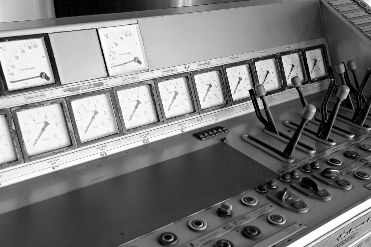
A curing oven takes fourteen minutes to reach setpoint. An incubator drifts a third of a degree over an hour. A 50-litre water bath has its sensor in a stainless pocket that answers a question you asked two minutes ago.
Tuning loops like these by feel is expensive, because every tweak costs a full thermal cycle before it teaches you anything. Change a gain, wait twenty minutes, shrug, change it again. Three hours later you have made a dozen changes and learned almost nothing.
There is a better sequence: measure the process once, calculate a sensible starting point, then refine with a small number of deliberate tests. Most of the work is waiting rather than fiddling.
Why slow thermal loops resist the usual methods
Three properties make ovens and incubators awkward. First, dead time. Heat has to travel from element to load, and the sensor sits somewhere in between, so the controller sees nothing for a while after it acts. Second, asymmetry. Heating is active and fast; cooling is passive, slow and dependent on ambient temperature, so a single set of gains is a compromise. Third, big time constants. A well-insulated chamber can take tens of minutes to settle, which means a test you would run in seconds on a motor takes half an hour here.
That combination punishes the classic ultimate-gain method, where you raise proportional gain until the loop oscillates and then back off. Deliberately oscillating a thermal process means cooking, freezing or spoiling whatever is inside it. Measure instead, and calculate.
Step one: prepare the experiment
Before touching a gain, get the conditions right. The measured response will be garbage if the chamber is being disturbed while you record it.
- Run the process at a representative operating point. Gains that behave at 40 °C may misbehave at 180 °C.
- Put the loop in manual and hold a steady output until the temperature is flat. Not "nearly flat" — flat.
- Keep doors shut, lids on, fans at their normal speed. A bench fan or an open window is a disturbance you will later blame on the controller.
- Log the data, ideally to a file rather than a phone photo of the display. One-second samples are plenty.
- Note your sample time and your output cycle time. A relay output time-proportioning over a 20-second window adds a delay you should know about. For solid-state relays, one or two seconds is usually ample.
Step two: measure the step response
From steady state, step the manual output by 10 to 20 % of range. Enough to see a clear move, small enough to stay in the roughly linear region and to avoid damaging the contents. Leave it alone and watch the curve until the temperature has flattened again, or until you have seen most of the transition. On a slow chamber that may mean recording for an hour, so start it early in the day.
Reading the numbers off the curve
You want three things. Dead time L: the delay between the step and the temperature first visibly moving. Time constant T: the time for the temperature to cover 63 % of its total change, or, more practically, the time from the start of the movement to the point where it settles. Gain K: the total temperature change divided by the output change, in matching units — for example, 6 °C rise from a 12 % output step gives 0.5 °C per percent.
If drawing tangents feels fussy, remember you only need accuracy good enough to get within a factor of two. Refinement does the rest.
Step three: calculate starting gains
For a self-regulating loop that behaves like dead time plus a single time constant, lambda tuning gives a clean, defensible start. Choose a closed-loop time constant λ — think of it as how briskly you want the loop to respond. A value roughly equal to the dead time is reasonably assertive; two to three times the dead time is gentle and safe.
- Proportional gain: Kc = T / (K × (λ + L))
- Integral time: Ti = T (in the same units as your measurements)
- Derivative: leave it at zero
Two warnings. First, integral units differ between controllers: seconds, minutes, minutes per repeat. If your manual wants repeats per minute, convert. Second, skip derivative on temperature loops. Sensor noise plus derivative action produces a jittery output and a short relay life, and the loop is too slow for derivative to earn its place.
For a well-insulated vessel with no meaningful heat loss, the response may look integrating rather than self-regulating — the temperature just keeps climbing. That needs a different rule set, and hunting for a steady state that never arrives will waste your afternoon.
Step four: test, then refine
Apply the calculated gains and make a setpoint step of a few percent of range. Log it. Then read the shape of the response.
- Slow creep towards setpoint, no overshoot: the loop is safe but lazy. Shorten Ti or increase Kc slightly.
- Overshoot followed by a long decay: integral is too aggressive for the dead time. Lengthen Ti.
- Sustained oscillation at a period of roughly four times the dead time: proportional gain is too high. Cut it by a third.
- Rapid jitter on the display: this is usually noise, not tuning. Filter the input or increase the sample time.
Change one thing at a time, and leave at least two full settling times between changes. Patience here is not virtue, it is throughput.
What tuning cannot repair
Some problems look like tuning and are not. A sensor clamped to the outside of a chamber reports the wall, not the load, and no gain fixes that. Long setpoint jumps cause overshoot on any slow loop; a setpoint ramp or a two-stage heat curve is often the honest solution. Insufficient insulation and draughty rooms produce wandering that a controller cannot outrun. And if the loop saturates at full output for a long time, integral windup will dump overshoot into your process — enable anti-windup, or hold the integrator while the output is clamped.
A routine worth repeating
Prepare the conditions, run one clean step test, extract L, T and K, calculate gains from λ, then refine with a handful of logged setpoint steps. Budget an afternoon for the first slow loop you tune this way; the second one goes much quicker, because you already know what a clean step response looks like on your rig. Keep the log files. When someone changes the insulation or the sensor next year, you will want to see what the loop used to do.
Photo: Şahin Sezer Dinçer / Pexels