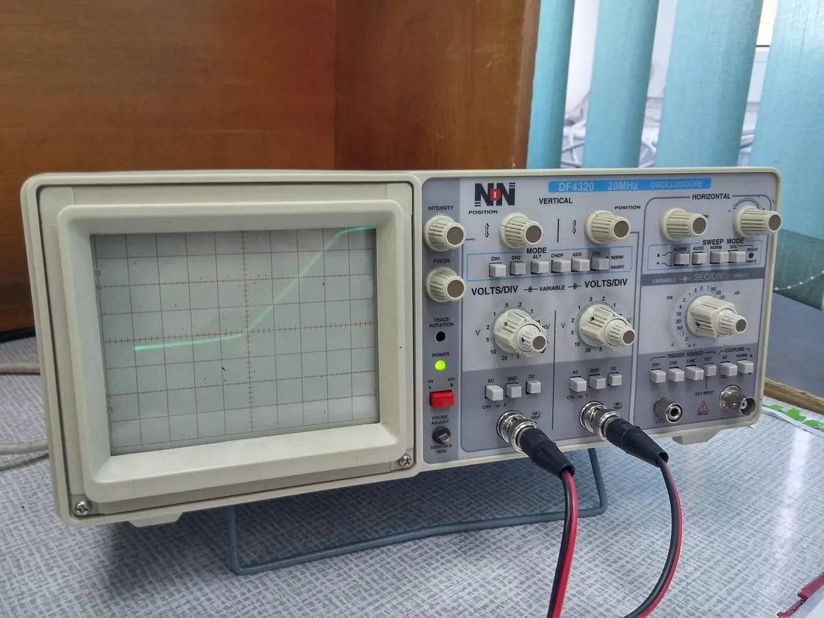
A temperature channel that swings up and down on a roughly 30-minute cycle, when nothing in the plant runs on a 30-minute cycle. A vibration spectrum with a sharp, repeatable peak at 200 Hz that no gear, bearing or shaft speed can explain. Both patterns turn up in real logs, both look convincing, and both are usually aliasing — an artefact created by the sampling itself.
Aliasing is the price of turning a continuous signal into numbers. Sample fast enough and the numbers describe the signal honestly. Sample too slowly and the high frequencies do not vanish politely; they reappear somewhere else on the frequency axis, looking exactly like genuine measurements.
What the Nyquist limit actually says
The Nyquist frequency is half your sample rate. Log once a second and it is 0.5 Hz; sample at 2 kHz and it is 1 kHz. The sampling theorem says that content above the Nyquist frequency will be misrepresented — not attenuated, not averaged away, misrepresented.
People often quote "sample at twice the highest frequency" as though it were a target. It is a mathematical minimum, and it assumes a perfect filter that does not exist. In practice you sample several times higher than the highest frequency you expect, and use a filter to deal with the content you did not expect.
Two terms get muddled, so keep them apart. The Nyquist frequency is fs/2, the highest frequency a given sample rate can represent. The Nyquist rate is the sample rate itself, and it must exceed twice the highest signal frequency.
How a signal folds back
An undersampled component does not simply disappear. It lands at a new frequency, given by folding: f_apparent = |f − n · fs|, where n is the integer that puts the result between 0 and fs/2.
Picture the frequency axis as a strip of paper marked from zero upwards, folded concertina-style at every multiple of the Nyquist frequency. Each band flips direction and lands on top of the band below. At a sample rate of 100 Hz, a 60 Hz tone folds to 40 Hz, a 140 Hz tone folds to 40 Hz, and a 160 Hz tone folds to 40 Hz as well. Three different signals, one apparent peak.
Worked example: a temperature log that follows a compressor
Take a thermocouple on a compressor discharge, logged every ten minutes to keep the file small. That is 1/600 Hz, so the Nyquist frequency is about 0.00083 Hz — a period of 20 minutes. Anything faster is invisible in the honest sense.
The compressor loads and unloads on a three-minute cycle, which is 0.0056 Hz, well above Nyquist. Fold it: 0.0056 ÷ 0.00167 = 3.33, so n = 3, and the alias is |0.0056 − 3 × 0.00167| = 0.00056 Hz. That is a period of about 30 minutes. The log now shows a tidy half-hourly oscillation in discharge temperature. It repeats, it survives averaging, and it looks like a control problem. It is a sampling artefact.
Mains interference behaves the same way, and often worse. A thermocouple amplifier with a bandwidth of tens of hertz will pass 50 Hz pickup quite happily. Log at 10 Hz and 50 Hz folds to 0 Hz — a DC shift that wanders with the mains, indistinguishable from a slow change in the process. Log the same channel at 12 Hz and the interference appears at 2 Hz instead. Same wiring, different alias.
Worked example: phantom peaks in vibration data
An accelerometer on a gearbox, sampled at 1 kHz, so the Nyquist frequency is 500 Hz. The shaft runs at 25 Hz and the gear mesh sits at 1.2 kHz. Fold it: 1200 − 1000 = 200 Hz. The second mesh harmonic at 2.4 kHz lands at 400 Hz.
Those two aliases look like the 8th and 16th shaft orders, and they are as sharp as real peaks. Engineers have spent days damping brackets and replacing bearings to remove components that were never in the machine. Aliases of real tones are coherent, which is the trap: random noise raises the noise floor, but an alias produces a clean peak, so it does not look like the mess people expect from interference.
Why you cannot filter an alias out afterwards
Once a component has folded, it occupies the same frequency range as genuine signal, and nothing downstream can tell the two apart. Digital low-pass filtering, decimation, averaging and smoothing all operate on samples you already have; the information needed to separate the alias was destroyed at the moment of conversion.
That is why anti-aliasing filters are analogue and sit immediately before the converter. A practical front end has an analogue low-pass with its cut-off comfortably below the Nyquist frequency, then, if you need fine resolution at low frequencies, a high sample rate followed by digital decimation.
Many loggers offer a "filter" or "averaging" setting that only smooths readings after sampling. Useful for a tidier trend line, useless against aliasing.
How to check whether you are looking at an alias
- Change the sample rate and re-measure. A real component stays at the same frequency; an alias moves. This one test settles most arguments.
- Do the arithmetic. Put the suspect frequency and your sample rate into the folding formula and see whether it predicts the peak on screen.
- Look for a mirrored family. Aliases of harmonics are regularly spaced too, but mirrored about the Nyquist frequency.
- Capture a short burst at the highest rate the hardware allows. A few seconds is usually enough to reveal what is really up there.
- Read the datasheet for the anti-aliasing filter. Ask what the attenuation is at the Nyquist frequency; 20 dB is not much.
Practical rules for setting up logging
Most aliasing is designed in, usually by choosing a sample rate to save disk space or match a display. A short checklist before you press record:
- List the highest frequency that could plausibly be present, not the one you care about — harmonics, gear mesh, PWM switching, supply ripple, mains pickup, sensor resonance.
- Set the sample rate to at least 2.5 times that figure, and five to ten times if the data will feed diagnostics.
- Confirm there is an analogue anti-aliasing filter ahead of the converter, with its cut-off below the Nyquist frequency and enough attenuation above it.
- Prefer oversampling with digital decimation over sampling at the bare minimum.
- Record the sample rate, filter cut-off and filter type with the data, so the next person can check whether a strange peak is real.
- Test once, deliberately: inject a known signal above the Nyquist frequency and see where it appears.
A tidy oscillation in a slow temperature log and a crisp peak in a vibration spectrum both deserve suspicion. Aliasing produces plausible data, which is exactly what makes it expensive. Set the rate from the physics, filter in analogue, and verify before you trust. If vibration data informs a safety decision about machinery, use an engineered measurement chain and take advice from a qualified condition-monitoring engineer.
Photo: 1837081 / Pixabay